

Process datasets and import results into Granta MI
Last update: 16.07.2025Load raw data from a .csv file and run a typical tensile data analysis to extract values for Ultimate Tensile Strength, Young's Modulus and Elongation at failure. Import the results into Granta MI.
Load data from CSV
The raw Load vs Displacement data is stored in a CSV file. Import the data directly into a DataFrame using the
pandas function .read_csv().
import pandas as pd

df_raw = pd.read_csv("supporting_files/04_raw_test_data.csv")
df_raw.head()
| Displacement [mm] | Load [N] | |
|---|---|---|
| 0 | 0.000000 | 0.000 |
| 1 | 0.005282 | 273.392 |
| 2 | 0.005282 | 307.173 |
| 3 | 0.006010 | 331.741 |
| 4 | 0.006738 | 352.556 |
The convention in this example is that all properties are in SI units unless otherwise specified. Create a new DataFrame, converting Displacement to SI units and renaming both columns.
df = pd.DataFrame()
df["Displacement"] = df_raw["Displacement [mm]"] / 1e3
df["Load"] = df_raw["Load [N]"]
df.head()
| Displacement | Load | |
|---|---|---|
| 0 | 0.000000 | 0.000 |
| 1 | 0.000005 | 273.392 |
| 2 | 0.000005 | 307.173 |
| 3 | 0.000006 | 331.741 |
| 4 | 0.000007 | 352.556 |
Process the data
Plot Load-Displacement data
This code snippet is optional, and is included to increase the size of all plots generated in this notebook.
import matplotlib.pyplot as plt

plt.rcParams["figure.dpi"] = 125
Use matplotlib to plot the Load-Displacement curve. For this plot, we've divided df.Load by 1e3 so the y-axis is
displayed in kN.
fig, ax = plt.subplots()
ax.plot(df.Displacement, df.Load / 1e3)
ax.set_xlabel("Displacement / m")
ax.set_ylabel("Load / kN")
_ = ax.set_title("Load vs displacement")

Convert Load-Displacement to Stress-Strain
Converting the Load-Displacement curve into Stress-Strain requires the gauge length and area, given here as constants in SI units. In a full workflow, these values can be loaded from a source file.
Calculate the Stress and Strain and store as new columns in the DataFrame.
GAUGE_WIDTH = 0.0150068
GAUGE_THICKNESS = 0.0015077
GAUGE_LENGTH = 0.07997724

df["Strain"] = df.Displacement / GAUGE_LENGTH
gauge_area = GAUGE_WIDTH * GAUGE_THICKNESS
df["Stress"] = df.Load / gauge_area
df.head()
| Displacement | Load | Strain | Stress | |
|---|---|---|---|---|
| 0 | 0.000000 | 0.000 | 0.000000 | 0.000000e+00 |
| 1 | 0.000005 | 273.392 | 0.000066 | 1.208322e+07 |
| 2 | 0.000005 | 307.173 | 0.000066 | 1.357626e+07 |
| 3 | 0.000006 | 331.741 | 0.000075 | 1.466210e+07 |
| 4 | 0.000007 | 352.556 | 0.000084 | 1.558207e+07 |
Now create a plot of Stress-Strain:
fig, ax = plt.subplots()
ax.plot(df.Strain, df.Stress / 1e6, zorder=0)
ax.set_xlabel(r"$\epsilon$")
ax.set_ylabel(r"$\sigma$ / MPa")
ax.set_xlim(left=0)
ax.set_ylim(bottom=0)

_ = ax.set_title("Stress vs Strain")
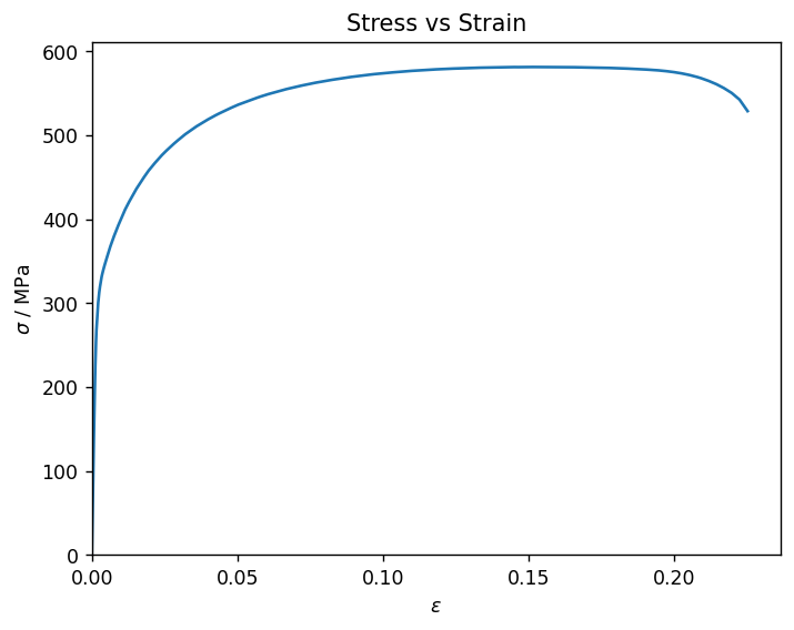
Since the plastic region extends over a large strain range, it is difficult to see detail in the elastic region.
Create an inset and plot the elastic and yield region only.
# [left, bottom, width, height] relative to the figure
ax_inset = fig.add_axes([0.25, 0.2, 0.4, 0.35])

ax_inset.plot(df.Strain, df.Stress / 1e6, label="Tensile response", zorder=0)
ax_inset.set_xlim(0, 0.004)
ax_inset.set_xticks([0, 0.004])

ax_inset.set_ylim(0, 400)
ax_inset.set_yticks([0, 400])

ax_inset.tick_params(axis="both", which="major", labelsize=8)
fig

Calculate Ultimate tensile strength
Ultimate tensile strength can be calculated by taking the maximum value of the df.Stress column.
Calculate and store the tensile strength in SI units and MPa (the latter will be used later).
tens_strength = df.Stress.max()
tens_strength_MPa = tens_strength / 1e6
print(f"Ultimate tensile strength: {tens_strength_MPa:.2f} MPa")
Previous cell output:
Ultimate tensile strength: 581.13 MPa
Add a marker and annotation on the stress-strain plot above, showing the location and value of the Ultimate tensile strength.
strain_at_uts = df.Strain[df.Stress == tens_strength].iloc[0]
ax.scatter(x=[strain_at_uts], y=[tens_strength_MPa], color="black", marker="x", alpha=0.75, s=50, zorder=1)
ax.annotate(rf"$\sigma_{{ts}}$: {tens_strength_MPa:.2f} MPa",
            xy=(strain_at_uts, tens_strength_MPa),
            xytext=(0,-14),
            textcoords="offset points",
            fontsize=8)
fig

Calculate Young's modulus
Calculate Young's modulus by taking the gradient of the Stress-Strain curve between 5% and 25% of the total tensile strength (chordal fit method). There is no interpolation, because the Stress-Strain values closest to the 5% and 25% bounds are used.
LOWER_FRACTION = 0.05
UPPER_FRACTION = 0.25

def get_stress_strain_at_fraction_of_tensile_strength(fraction):
    stress_bound = tens_strength * fraction
    stress_difference = df.Stress - stress_bound
    nearest_row_number = stress_difference.abs().argsort()[0]
    nearest_row = df.iloc[nearest_row_number]
    return nearest_row.Strain, nearest_row.Stress

lower_strain, lower_stress = get_stress_strain_at_fraction_of_tensile_strength(LOWER_FRACTION)
upper_strain, upper_stress = get_stress_strain_at_fraction_of_tensile_strength(UPPER_FRACTION)

youngs_modulus = (upper_stress - lower_stress) / (upper_strain - lower_strain)
print(f"Young's modulus ({LOWER_FRACTION:.0%}-{UPPER_FRACTION:.0%} tensile strength): {youngs_modulus / 1e9:.2f} GPa")
Previous cell output:
Young's modulus (5%-25% tensile strength): 204.65 GPa
Add the chordal fit to the inset plot.
stress_linear_fit = df.Strain * youngs_modulus
ax_inset.plot(df.Strain, stress_linear_fit / 1e6, "r--", label="Young's modulus", zorder=-1)

fig

Calculate 0.2% offset yield stress
The offset yield stress is determined by calculating the intercept between the chordal fit line and the stress response.
First add the offset chordal fit line to the plot, to show where the yield stress lies.
STRAIN_OFFSET = 0.002

strain_offset = df.Strain + STRAIN_OFFSET
ax_inset.plot(strain_offset, stress_linear_fit / 1e6, "k:", label="0.2% offset", zorder=-1)

handles, labels = ax_inset.get_legend_handles_labels()
legend_position = (0.575, 0.85)
ax.legend(handles, labels, bbox_to_anchor=legend_position, prop={"size": 8})
fig

Calculate the difference between the solid blue and dotted black lines, then find the values immediately before and after the intercept. Perform a linear interpolation to find the exact value of the yield stress.
df["find_intercept"] = df.Stress - youngs_modulus * (df.Strain - STRAIN_OFFSET)
first_row_index_above_intercept = (
    df
    .loc[df.find_intercept  0]
    .sort_values(by=["find_intercept"], ascending=False)
    .index[0]
)
y_1 = df.Stress.iloc[first_row_index_above_intercept]
x_1 = df.find_intercept.iloc[first_row_index_above_intercept]

last_row_index_below_intercept = (
    df
    .loc[df.find_intercept >= 0]
    .sort_values(by=["find_intercept"], ascending=True)
    .index[0]
)
y_0 = df.Stress.iloc[last_row_index_below_intercept]
x_0 = df.find_intercept.iloc[last_row_index_below_intercept]

yield_stress = y_0 + (-x_0) * (y_1 - y_0) / (x_1 - x_0)
strain_at_yield = yield_stress / youngs_modulus + STRAIN_OFFSET

yield_stress_MPa = yield_stress / 1e6
print(f"0.2% offset yield stress: {yield_stress_MPa:.2f} MPa")
Previous cell output:
0.2% offset yield stress: 335.56 MPa
Plot the 0.2% offset yield stress on the Stress-Strain plot. This time, plot the marker on both the full and inset axes, and annotate the inset.
ax.scatter(
    x=[strain_at_yield],
    y=[yield_stress_MPa],
    color="black",
    marker="1",
    alpha=0.75,
    s=50,
    zorder=1,
)
ax_inset.scatter(
    x=[strain_at_yield],
    y=[yield_stress_MPa],
    color="black",
    marker="1",
    alpha=0.75,
    s=50,
    zorder=1,
)
ax_inset.annotate(
    rf"$\sigma_y$: {yield_stress_MPa:.2f} MPa",
    xy=(strain_at_yield, yield_stress_MPa),
    xytext=(-60,6),
    textcoords="offset points",
    fontsize=8)
fig

Calculate Elongation at failure
The data has been pre-processed before import, so the last point in the data series is the failure point.
stress_at_break = df.Stress.iloc[-1]
total_strain_at_break = df.Strain.iloc[-1]
elastic_strain_at_break = stress_at_break / youngs_modulus
elongation = total_strain_at_break - elastic_strain_at_break
print(f"Elongation at failure: {elongation:.2%}")
Previous cell output:
Elongation at failure: 22.27%
Plot the Elongation at failure on the full-range axes, and add a line between the failure point and the elongation value. The legend updates to include all lines on both sets of axes.
ax.plot(
    [total_strain_at_break, elongation],
    [stress_at_break / 1e6, 0],
    "y-.",
    label="Elongation",
    zorder=-1,
)
ax.scatter(
    x=[total_strain_at_break, elongation],
    y=[stress_at_break / 1e6, 0],
    color="black",
    marker="2",
    alpha=0.75,
    s=50,
    zorder=1,
)

inset_handles, inset_labels = ax_inset.get_legend_handles_labels()
ax_handles, ax_labels = ax.get_legend_handles_labels()
handles = inset_handles + ax_handles
labels = inset_labels + ax_labels
ax.get_legend().remove()
ax.legend(handles, labels, bbox_to_anchor=legend_position, prop={"size": 8})

ax.annotate(
    rf"$\epsilon_f$: {elongation:.3}",
    xy=(elongation, 0),
    xytext=(-40,5),
    textcoords="offset points",
    fontsize=8,
)
fig

Calculate True Stress-Strain
Since there is a 1:1 relationship between engineering and true stress-strain values, True Stress-Strain is added to the DataFrame as additional columns.
import numpy as np

ts_position = df.Stress[df.Stress == tens_strength].index[0]

# true strain = ln(1 + eng strain)
df["True_Strain"] = np.log(1 + df.Strain[df.Strain.index = ts_position])

# true stress = eng stress * (1 + eng strain)
df["True_Stress"] = df.Stress[df.Stress.index = ts_position] * (1 + df.True_Strain)
df.head()
| Displacement | Load | Strain | Stress | find_intercept | True_Strain | True_Stress | |
|---|---|---|---|---|---|---|---|
| 0 | 0.000000 | 0.000 | 0.000000 | 0.000000e+00 | 4.093098e+08 | 0.000000 | 0.000000e+00 |
| 1 | 0.000005 | 273.392 | 0.000066 | 1.208322e+07 | 4.078764e+08 | 0.000066 | 1.208402e+07 |
| 2 | 0.000005 | 307.173 | 0.000066 | 1.357626e+07 | 4.093694e+08 | 0.000066 | 1.357715e+07 |
| 3 | 0.000006 | 331.741 | 0.000075 | 1.466210e+07 | 4.085924e+08 | 0.000075 | 1.466320e+07 |
| 4 | 0.000007 | 352.556 | 0.000084 | 1.558207e+07 | 4.076494e+08 | 0.000084 | 1.558338e+07 |
Create a new plot to compare Engineering and True Stress-Strain.
fig, ax = plt.subplots()
ax.plot(
    df.Strain,
    df.Stress / 1e6,
    label="Engineering Stress",
    linestyle="--",
)
ax.plot(
    df.True_Strain,
    df.True_Stress / 1e6,
    label="True Stress",
)
ax.set_xlabel(r"$\epsilon$")
ax.set_ylabel(r"$\sigma$ / MPa")
ax.set_xlim(left=0)
ax.set_ylim(bottom=0)
ax.legend()
_ = ax.set_title("Engineering and True Stress vs Strain")

Calculate True Stress-True Plastic Strain
Create a new DataFrame to store the True Stress-True Plastic Strain, since the x-axis is different to Stress-Strain.
df_plastic = pd.DataFrame()
plastic_strain = df.True_Strain - df.True_Stress / youngs_modulus - STRAIN_OFFSET
df_plastic["Strain"] = plastic_strain[plastic_strain > 0]

# Get only the stress values with a corresponding strain
df_plastic["Stress"] = df.True_Stress.align(df_plastic.Strain, join='right')[0]

# Manually add the first point Strain = 0, Stress = yield stress
first_point = pd.DataFrame({"Strain": [0], "Stress": [yield_stress]})
df_plastic = pd.concat([first_point, df_plastic], ignore_index=True)
df_plastic.head()
| Strain | Stress | |
|---|---|---|
| 0 | 0.000000 | 3.355557e+08 |
| 1 | 0.000008 | 3.370594e+08 |
| 2 | 0.000029 | 3.374152e+08 |
| 3 | 0.000050 | 3.377409e+08 |
| 4 | 0.000067 | 3.380495e+08 |
Plot True Stress-True Plastic Strain. Force the x limit to be 0, but not the y limit (the curve starts at the Yield stress).
df_plastic["Stress_MPa"] = df_plastic.Stress / 1e6

fig, ax = plt.subplots()
ax.plot(df_plastic.Strain, df_plastic.Stress_MPa, label="True Stress")
ax.set_xlabel(r"$\epsilon$")
ax.set_ylabel(r"$\sigma$ / MPa")
ax.set_xlim(left=0)
_ = ax.set_title("True Stress vs True Plastic Strain")

Import data and results into Granta MI
Finally, import the raw data, processed data and results into a new Granta MI record.
Connect to Granta MI and specify a database and table.
from GRANTA_MIScriptingToolkit import granta as mpy

mi = mpy.connect("http://my.server.name/mi_servicelayer", autologon=True)
db = mi.get_db(db_key='MI_Training')

tensile_test_table = db.get_table('Tensile Test Data')
Create a new record to import the data into, using datetime.now() to ensure the record name is unique.
At this stage, the record has only been created in the MI Scripting Toolkit. The changes will be pushed to Granta MI
when session.update() is called at the end of the notebook.
from datetime import datetime

now = datetime.now().strftime("%c")
record_name = f"Tensile analysis {now}"

folder = tensile_test_table.path_from(starting_node=None, tree_path=["Data Analytics"])
record = tensile_test_table.create_record(name=record_name, parent=folder)
Create and populate point attributes
Define a function to write a dict of attribute name-value pairs to point attributes on the record. Each dict will contain values with a single unit.
def write_points(attrs, unit):
    for name, value in attrs.items():
        a = record.attributes[name]
        a.value = value
        a.unit = unit
        record.set_attributes([a])
Build the dicts of attribute name-value pairs and call the function above on each. (The strain values are dimensionless but will be imported as a percentage, so they are multiplied by 100 before import.)
stress_attrs = {
    "Ultimate Tensile Strength": tens_strength,
    "Young's Modulus (11-axis)": youngs_modulus,
    "0.2% Offset Yield Stress": yield_stress
}
strain_attrs = {
    "Strain at Ultimate Tensile Strength": strain_at_uts * 100,
    "Elongation": elongation * 100,
    "Strain at Tensile Failure": total_strain_at_break * 100,
}
length_attrs = {
    "Gauge Length": GAUGE_LENGTH,
    "Gauge Width": GAUGE_WIDTH,
    "Gauge Thickness": GAUGE_THICKNESS,
}
area_attrs = {"Gauge Area": gauge_area}

write_points(stress_attrs, "Pa")
write_points(strain_attrs, "%")
write_points(length_attrs, "m")
write_points(area_attrs, "m^2")
Create and populate text attributes
Define a similar function for text attributes:
def write_text(attrs):
    for name, value in attrs.items():
        a = record.attributes[name]
        a.value = value
        record.set_attributes([a])
Define the dict of text attributes, and call the function above. We've defined the attribute values manually, but they could easily be read from the source file.
range_text = f"Linear fit between [{LOWER_FRACTION:.1%}:{UPPER_FRACTION:.1%}] of Tensile strength"
text_attrs = {
    "Young's Modulus Calculation": 'Chord',
    "Test Type": 'Tensile',
    "Testing Standards": 'ASTM E8',
    "Alloy": 'AMS 6520',
    "Modulus Calculation Range": range_text,
}
write_text(text_attrs)
Create and populate functional attributes
Finally, define a function to import functional attributes.
def write_functional(attr_name, y_unit, x_unit, x_name, y_values, x_values):
    a = record.attributes[attr_name]
    a.unit = y_unit
    a.parameters[x_name].unit = x_unit
    a.xaxis[x_name] = True
    for x, y in zip(x_values, y_values):
        a.add_point({'y': y, x_name: x})
    record.set_attributes([a])
Call the function for each curve generated in this script.
write_functional(
    attr_name="Load vs Displacement",
    y_unit="N",
    x_unit="m",
    x_name="Displacement",
    y_values=df.Load,
    x_values=df.Displacement,
)

write_functional(
    attr_name="Tensile Response (11 axis)",
    y_unit="Pa",
    x_unit="strain",
    x_name="Strain",
    y_values=df.Stress,
    x_values=df.Strain,
)

write_functional(
    attr_name="True Stress vs True Plastic Strain",
    y_unit="Pa",
    x_unit="strain",
    x_name="Strain",
    y_values=df_plastic.Stress,
    x_values=df_plastic.Strain,
)
Write your changes to Granta MI
mi.update([record])
Previous cell output:
[<record long name: tensile analysis mon may>]