

Pipe mapping tutorial
Last update: 09.03.2026This tutorial gives instructions on using System Coupling Participant Library APIs to transfer data across a non-conformal mesh interface, thereby using the participant library mapping capabilities.
The tutorial also demonstrates how to use parallel processing capabilities within the Participant Library using an MPI environment.
Topics covered
- Standalone mapping
- Parallel execution
Verify prerequisites
Ensure that the following prerequisites are met. You have the following:
-
Ansys installation, including System Coupling and EnSight.
-
A compiler for one of the supported languages
- This is only a requirement if you need to compile the application. Pre-compiled executables are provided, along with a Python script.
Problem description and participant setup
In this example, we transfer the data between two regions representing a simple pipe geometry.
Each of the two regions is meshed using a different method, so that we generate the non-conformal mesh interface. The first region, quad, is meshed using an algorithm that generates mesh with quadrilateral elements. The second region, tri, is meshed using an algorithm that generates mesh with trilateral elements. The meshes with default settings are shown in Figure 1.
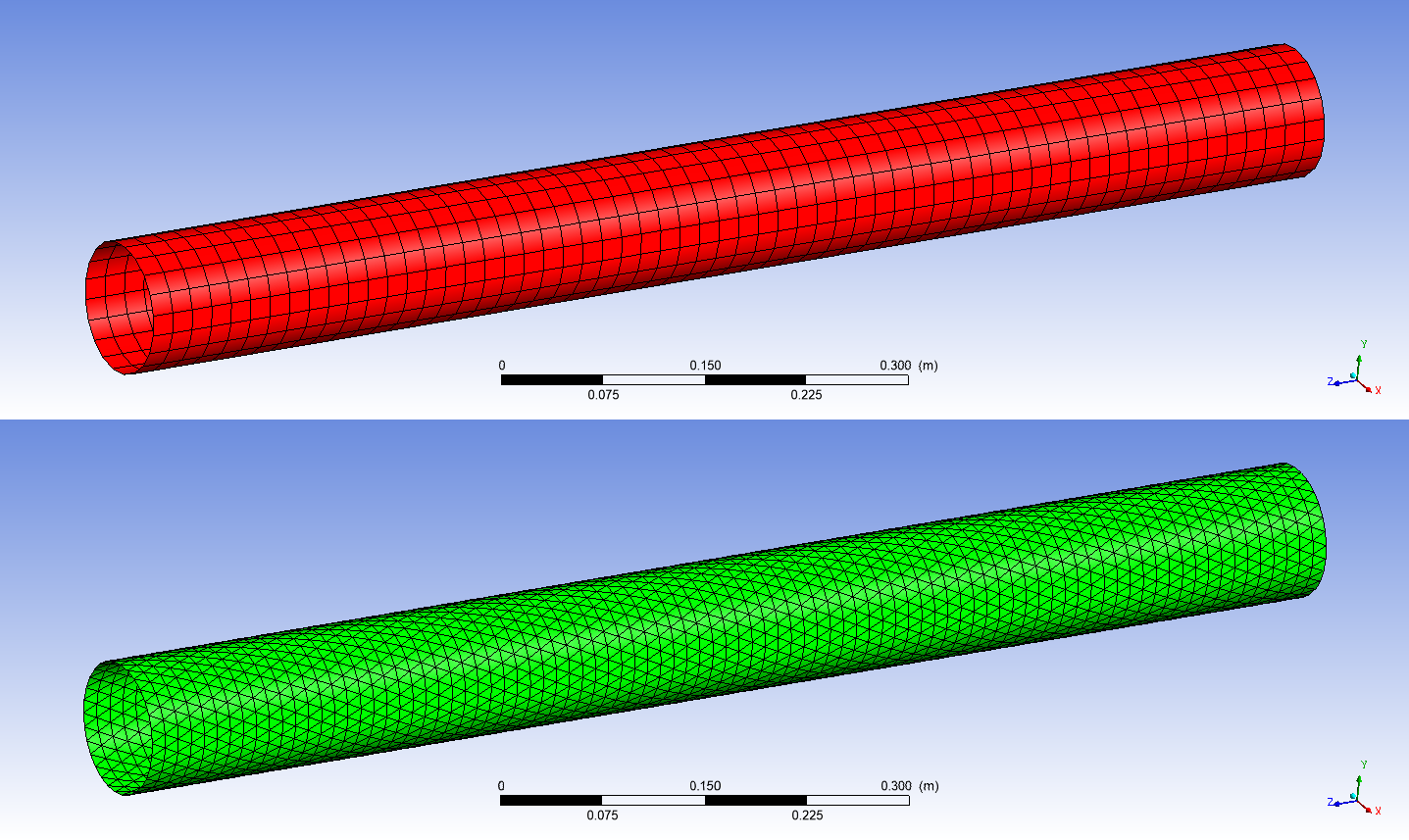
Figure 1: Default pipe meshes
On each side, we initialize the nodal solution data with a simple linear profile $f(x,y,z) = 1x + 2y + 3z + 4$. On the quad region, we initialize quadProfile variable, and on the tri region, we initialize the triProfile variable.
We then use the mapping capabilities within the Participant Library to transfer quadProfile data from quad to tri region, and also to transfer triProfile data from tri to quad region.
Finally, we make use of the writeResults API function to write the results
for further post-processing. These results can be visualized in Ansys EnSight.
Overview of the pipe mapping program and accompanying scripts
We provide the source code to generate a simple program that:
- Generates the meshes
- Initializes the solution data
- Implements the Participant Library APIs to set up and execute the mapping
- Exports the resulting data for further post-processing
The source code for each of the supported languages is provided with the tutorial package. A serial implementation is provided in Python, while parallel implementations are provided in C++, C, and Fortran. C++ implementation provides some additional functionality, not available in other languages.
The code to generate the mesh and to initialize the solution data
is implemented in the separate file(s) and is called PipeMeshGenerator module.
The implementation details of how the meshes are generated can be skipped
(initializeMesh() and associated functions/subroutines).
Most of the System Coupling Participant Library APIs are contained
inside the main source code file (PipeMapping.cpp, PipeMapping.c,
PipeMapping.f90, or PipeMapping.py).
Several command-line arguments can be used to customize the problem. Mesh refinement for the quad region can be controlled as follows:
--quad N (default N = 20)
where N is the refinement number. The pipe mesh will have N edges in
circumferential direction and 3*N edges in the axial direction. An analogous
command-line argument can be used to control the refinement of the tri
region:
--tri N (default N = 30)
The quad region can be offset in the axial direction using the following command-line argument:
--offset Z (default Z = 0.0)
The pipe radius for quad and tri regions can be controlled by the following command-line arguments, respectively:
--qradius R (default R = 0.05)
--tradius R (default R = 0.05)
For the parallel implementation, the mesh is partitioned using a recursive binary space partitioning algorithm. The pipe is recursively sub-divided in either axial or circumferential directions, depending on which direction is longer. Figure 2 demonstrates how the quad region is divided when 7 partitions are used.
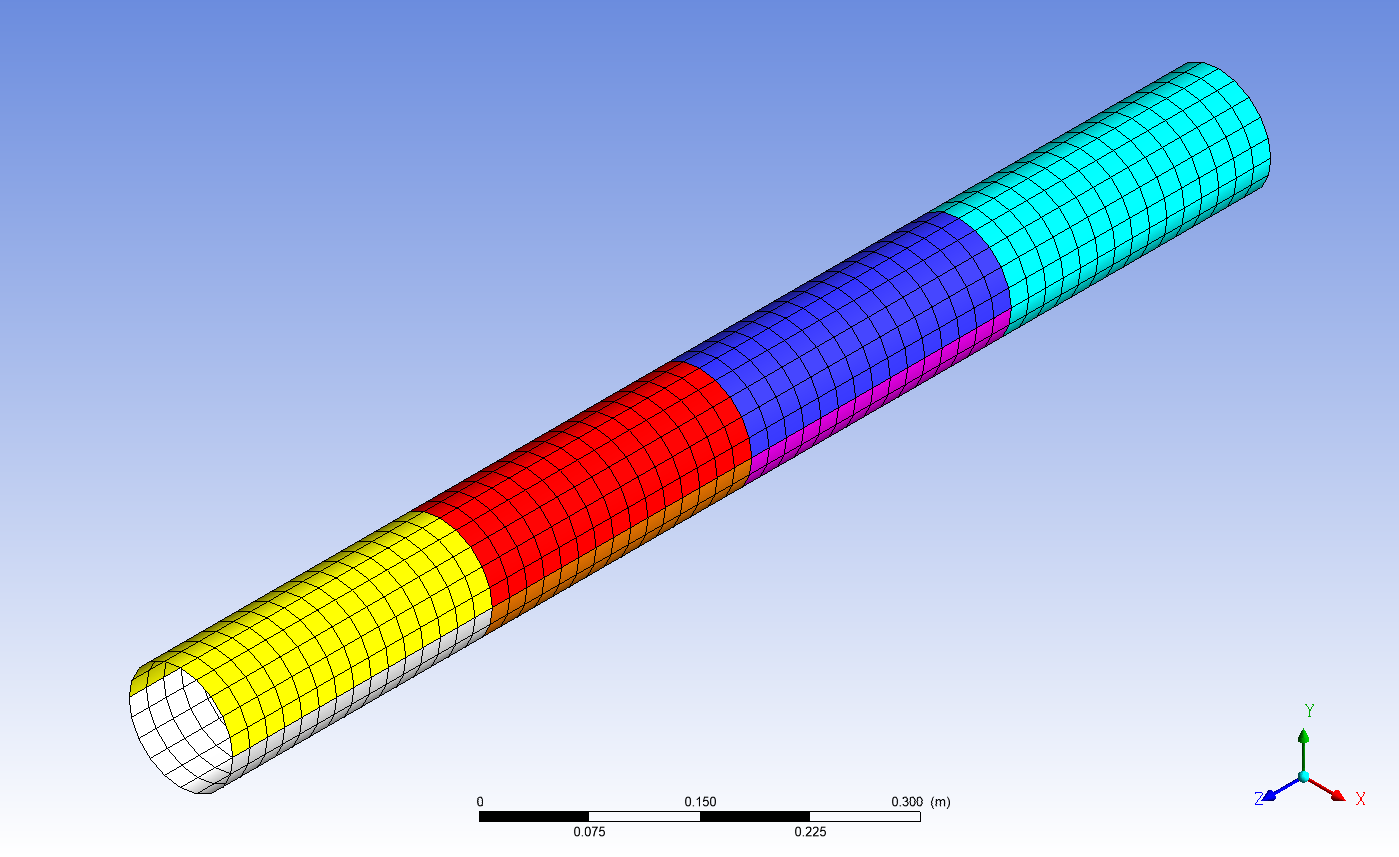
Figure 2: Sample partitioning
After mapping, the mesh and resulting solution data can be written to the EnSight results files for visualization. To control whether the results files are written, use the following command-line argument:
--write W (W = 1 means write, W = 0 means do not write, default W = 1)
--elemdata E (C++ only) (E = 0 means nodal data, E = 1 means element data, default E = 0)
The Pipe Mapping program uses a wrapper script (PipeMapping.bat for Windows,
PipeMapping.sh for Linux), that sets up the required environment variables and
controls parallel execution. Th Pipe Mapping program that is written in Python
has different execution requirements than those written in C++, C, or Fortran,
so for Python a separate set of wrapper scripts is provided
(PipeMappingPython.bat for Windows, PipeMappingPython.sh for Linux).
More examples of how to execute the Pipe Mapping program and the accompanying Python post-processing script are shown in subsequent sections of this tutorial.
Get the necessary files
Download the SCP library tutorial package and extract it to a local directory. Inside the resulting directory, you will find a subdirectory called PipeMapping. This directory contains all the files needed for this tutorial. The contents of this subdirectory are:
-
src_c: Directory containing the C source code files:
PipeMapping.c: C Pipe Mapping program code and explanatory comments.PipeMeshGenerator.c: The C implementation file for the Pipe Mesh Generator module.PipeMeshGenerator.h: The C header file for the Pipe Mesh Generator module.
-
src_cpp: Directory containing the C++ source code files:
PipeMapping.cpp: The Pipe Mapping program C++ source code file.PipeMeshGenerator.cpp: The C++ implementation file for the Pipe Mesh Generator module.PipeMeshGenerator.hpp: The C++ header file for the Pipe Mesh Generator module.
-
src_fortran: Directory containing the Fortran source code files:
PipeMapping.f90: The Pipe Mapping program Fortran source code file.PipeMeshGenerator.f90: The Fortran source code file for the Pipe Mesh Generator module.
-
PipeMapping: Linux binary executable for the Pipe Mapping program. -
PipeMapping.bat: Windows batch script for executing the Pipe Mapping program and writing the output files. -
PipeMapping.exe: Windows binary executable for the Pipe Mapping program. -
PipeMapping.py: Python Pipe Mapping program code and explanatory comments. -
PipeMapping.sh: Linux shell script for executing the Pipe Mapping program and writing the output files. -
PipeMappingPython.bat: Windows batch script for executing the Python Pipe Mapping program and writing the output files. -
PipeMappingPython.sh: Linux shell script for executing the Python Pipe Mapping program and writing the output files. -
PipeMeshGenerator.py: The Python source code file for the Pipe Mesh Generator module.
Build the pipe mapping program
Build the Pipe Mapping program using a compiler for one of the supported languages.
Note: Pre-built executables are provided along with the source code, so this step is optional.
Note: For Python, the Pipe Mapping script does not need to be compiled, so this step can be skipped.
In the following examples, Pipe Mapping programs are built with different configurations. The actual build steps depend on your system configuration, compilers, and other details. For additional information, see Compiling, Linking, and Executing Applications That Use the Participant Library in the Participant Library Developer's Guide.
The following compilers were used in these examples:
- Linux
- GNU (g++, gcc, and gfortran) 8.2.0
- Windows
- Microsoft (R) C/C++ Optimizing Compiler Version 19.16.27040 for x64
- Intel(R) Visual Fortran Intel(R) 64 Compiler Version 19.0.4.245
In the following examples, replace:
<ANSYSInstallationPath>with the correct Ansys installation path<MultiportVersion>with the correct version of the Fluent Multiport library<IntelMPIPath>with the correct path to the Intel MPI library
Linux
C++ parallel version using Intel MPI
g++ -std=c++11 -I<ANSYSInstallationPath>/SystemCoupling/runTime/linx64/include -I<IntelMPIPath>/intel64/include -L<ANSYSInstallationPath>/SystemCoupling/runTime/linx64/bin -L<IntelMPIPath>/intel64/lib/release -L<ANSYSInstallationPath>/SystemCoupling/runTime/linx64/bin -L<ANSYSInstallationPath>/SystemCoupling/runTime/linx64/cnlauncher/fluent/fluent<MultiportVersion>/multiport/mpi_wrapper/lnamd64/stub -o PipeMapping src_cpp/PipeMeshGenerator.cpp src_cpp/PipeMapping.cpp -lSysC.SystemCouplingParticipant -lmpi -lmpi_wrapper
C parallel version using Intel MPI
gcc -I<ANSYSInstallationPath>/SystemCoupling/runTime/linx64/include -I<IntelMPIPath>/intel64/include -L<ANSYSInstallationPath>/SystemCoupling/runTime/linx64/bin -L<IntelMPIPath>/intel64/lib/release -L<ANSYSInstallationPath>/SystemCoupling/runTime/linx64/bin -L<ANSYSInstallationPath>/SystemCoupling/runTime/linx64/cnlauncher/fluent/fluent<MultiportVersion>/multiport/mpi_wrapper/lnamd64/stub -o PipeMapping src_c/PipeMeshGenerator.c src_c/PipeMapping.c -lSysC.SystemCouplingParticipant -lmpi -lmpi_wrapper -lm
Fortran parallel version using Intel MPI
gfortran -I<ANSYSInstallationPath>/SystemCoupling/runTime/linx64/include/SystemCouplingParticipant/FortranFreeForm -I<IntelMPIPath>/intel64/include -L<ANSYSInstallationPath>/SystemCoupling/runTime/linx64/bin -L<IntelMPIPath>/intel64/lib -L<IntelMPIPath>/intel64/lib/release -L<ANSYSInstallationPath>/SystemCoupling/runTime/linx64/cnlauncher/fluent/fluent<MultiportVersion>/multiport/mpi_wrapper/lnamd64/stub -o PipeMapping src_fortran/PipeMeshGenerator.f90 src_fortran/PipeMapping.f90 -lSysC.SystemCouplingParticipant.Fortran -lmpifort -lmpi -lmpi_wrapper
Windows
C++ parallel version using Intel MPI
cl /EHsc /I"<ANSYSInstallationPath>\SystemCoupling\runTime\winx64\include" /I"<IntelMPIPath>\intel64\include" src_cpp\PipeMeshGenerator.cpp src_cpp\PipeMapping.cpp /FePipeMapping.exe /link /subsystem:console /LIBPATH:"<ANSYSInstallationPath>\SystemCoupling\runTime\winx64\lib" SysC.SystemCouplingParticipant.lib /LIBPATH:"<IntelMPIPath>\intel64\lib" impi.lib
C parallel version using Intel MPI
cl /EHsc /I"<ANSYSInstallationPath>\SystemCoupling\runTime\winx64\include" /I"<IntelMPIPath>\intel64\include" src_c\PipeMeshGenerator.c src_c\PipeMapping.c /FePipeMapping.exe /link /subsystem:console /LIBPATH:"<ANSYSInstallationPath>\SystemCoupling\runTime\winx64\lib" SysC.SystemCouplingParticipant.lib /LIBPATH:"<IntelMPIPath>\intel64\lib" impi.lib
Fortran parallel version using Intel MPI
ifort -I"<ANSYSInstallationPath>\SystemCoupling\runTime\winx64\include\SystemCouplingParticipant\FortranFreeForm" -I"<IntelMPIPath>\intel64\include" /FePipeMapping.exe src_fortran\PipeMeshGenerator.f90 src_fortran\PipeMapping.f90 /link /subsystem:console /LIBPATH:"<ANSYSInstallationPath>\SystemCoupling\runTime\winx64\lib" SysC.SystemCouplingParticipant.Fortran.lib /LIBPATH:"<IntelMPIPath>\intel64\lib" impi.lib
Execute the pipe mapping program using the default settings
The Pipe Mapping application can be executed from the command console, as shown below, depending on the platform and the implementation language.
Windows
Execute from the Command Prompt.
Pipe mapping program (non-Python)
PipeMapping.bat
Python pipe mapping program
PipeMappingPython.bat
Linux
Execute from the shell.
Pipe mapping program (non-Python)
./PipeMapping.sh
Python pipe mapping program
./PipeMappingPython.sh
Note: For the sake of brevity, the rest of this tutorial assumes the use of the Linux platform and non-Python implementation.
This will execute the Pipe Mapping program, generate the .dat files, read them into the
provided Python script, generate the .axdt files, and then delete the .dat files.
The program will also print some diagnostics information (such as timing information for various functions) to the console and report the maximum error on each region. Example expected output:
Setup:
Quad refinement: 20
Tri refinement: 30
Pipe offset: 0
Quad radius: 0.05
Tri radius: 0.05
Write: 1
Overlap layers: 0
Processes: 1
==========
Time to generate mesh: 1.5522e-03 [s]
Time to update inputs: 1.1918e-01 [s]
Time to write results: 6.3139e-03 [s]
Maximum error on quad: 6.2552e-04
Maximum error on tri: 1.2232e-03
Note: The batch and the shell scripts use the environment variable
AWP_ROOT<version>to set up the participant solver environment. Make sure this environment variable is set to the Ansys installation path (for exampleC:\Program Files\ANSYS Inc\v<version>). Alternatively, you can modify the scripts to use a different environment variable.***
Visualize the results in Ansys EnSight
Use Ansys EnSight to view the results produced by the Pipe Mapping program. You'll be able to visualize the pipe mesh and nodal profile of the quadProfile and triProfile variables.
-
Open Ansys EnSight.
-
Load the pipe mapping results.
a. In the EnSight menu toolbar, select File > Open.
b. In the Open... dialog, select Multiple file interface.
c. Select the results files that were generated when the Pipe Mapping program was executed:
pipe.caseif running in serial, orpipe_*.caseif running in parallel (hold theCtrlkey when selecting multiple files). Click Add to list button.d. Select Load all parts.
The pipe mapping results files are loaded and the geometry is displayed on the EnSight's viewer.
e. Click View > Hidden line and check the Specify the line overlay color checkbox.
The mesh lines are shown in EnSight's viewer.
-
Plot the mapped triProfile variable profile on the quad region.
a. In the Parts pane, de-select the Show check-box for
triand select the check-box forquad.b. In the Variables pane, activate the triProfile variable (enable the Activate checkbox).
c. In the Variables pane, right-click the triProfile variable and select Color parts > Selected.
The profile of the mapped triProfile variable on the quad region is shown in the viewer.
-
Plot the mapped quadProfile variable profile on the tri region.
a. In the Parts pane, de-select the Show checkbox for
quadand select the checkbox fortri.b. In the Variables pane, activate the quadProfile variable (enable the Activate checkbox).
c. In the Variables pane, right-click on the quadProfile variable and select Color parts > Selected.
The profile of the mapped quadProfile variable on the tri region is shown in the viewer.
Figure 3 shows the resulting plots. Note that the contours of the profiles are virtually identical in both regions.
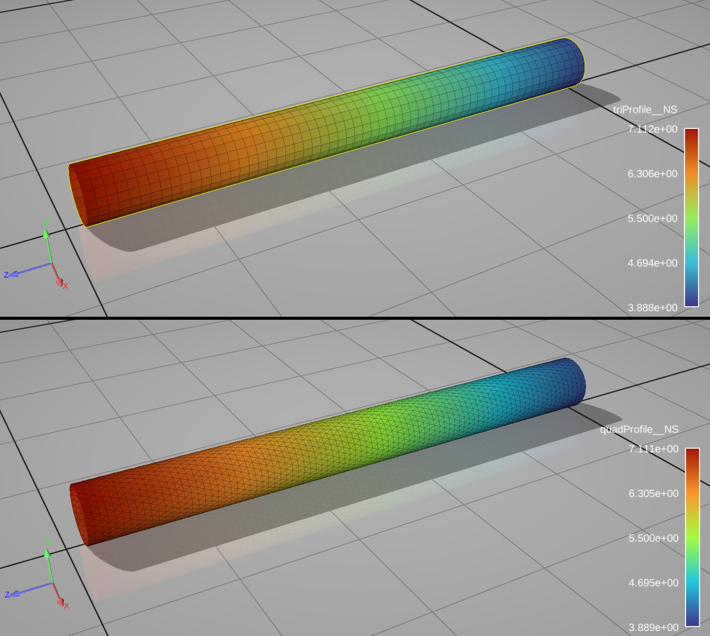
Figure 3: Nodal solution data profiles for the mapped variables
Run and post-process the results using the provided customization settings
Various customization settings can be used. In each case, the post-processing step to visualize the .axdt files is the same.
Mesh refinement
To refine the mesh on both quad and tri regions, re-run the pipe mapping as follows:
./PipeMapping.sh --quad 100 --tri 150
Figure 4 shows the resulting mesh and solution profiles in EnSight.
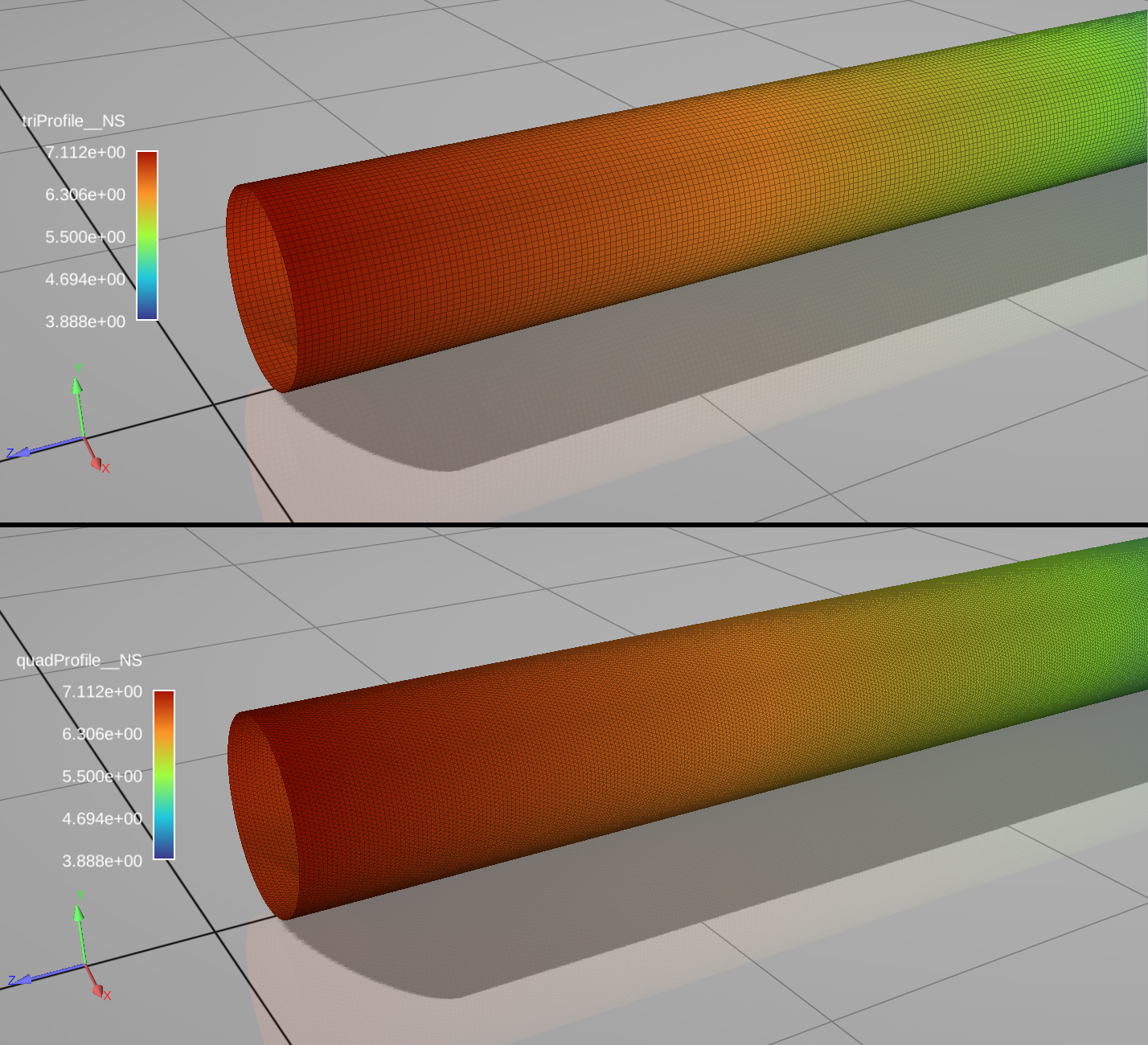
Figure 4: Solution profiles on refined meshes
Parallel execution
Note: Parallel execution using Python is not supported, so this section only applies to Pipe Mapping programs compiled from C++, C, or Fortran.
In this step, the Pipe Mapping program will be run using local parallel execution. The Intel MPI distribution that comes with System Coupling will be used to execute the Pipe Mapping program. In this example, the program will be executed using 4 processes:
./PipeMapping.sh -np 4
Parallel overlap layer can be inserted using --overlap command line argument. For instance,
to create an overlap of two elements on each partition bundary:
./PipeMapping.sh -np 4 --overlap 2
The final results will be identical, regardless of the number of parallel processes used, and of the number of elements in the overlap layer.
The Pipe Mapping program can also be executed in a distributed parallel environment, including execution on a High-Performance Computing (HPC) cluster. The details of how to set up the environment for distributed parallel execution are beyond the scope of this tutorial. Assuming that the environment is set up appropriately, suppose we want to execute the program on 2 hosts (for example, hostA and hostB), with each having 4 cores available. In this case, the Pipe Mapping program can be executed as follows:
./PipeMapping.sh -hostlist hostA:4,hostB:4
Order of accuracy calculation
We can demonstrate that the mapping algorithm preserves 2nd order of accuracy of the mapped profile. We use C++ implementation to demonstrate the 2nd order accuracy is preserved when data is on nodes (default) and also when the data is on element centroids.
Both source and target meshes are refined simultaneously. The element area is found by dividing the analytical area of the pipe by the number of elements. The element size is then determined by taking the square root of the element area.
Plugging the pipe mapping program into the following Python script allows running multiple instances with with various levels of refinements. We then parse out the maximum error and calculate the slope of error vs. mesh size. We confirm that the slope of the logarithmic plot is approximately 2.0, which means that the mapping algorithms preserve 2nd order mapping accuracy.
import math
import subprocess
import sys
import scipy.stats


def getExe():
    ext = "bat"
    if sys.platform != "win32":
        ext = "sh"
    return f"PipeMapping.{ext}"


def getArgs(refine: int, isElem: bool):
    args = f"--write 0 --quad {refine} --tri {refine}"
    if isElem:
        args += " --elemdata"
    return args


def getQuadError(output: tuple) -> float:
    outputStr = str(output[0])
    splitToken = r"\r\n"
    if sys.platform != "win32":
        splitToken = r"\n"
    tokens = outputStr.split(splitToken)
    quadErrorLine = [t for t in tokens if "Maximum error on quad" in t][0]
    return float(quadErrorLine.split(": ")[1])


def getSlope(refinements, quadErrors) -> float:
    def getElemSize(refinement):
        return math.sqrt(2.0 * math.pi * 0.05 / (refinement * refinement * 3.0))

    elemSizes = [getElemSize(r) for r in refinements]
    logSizes = [math.log10(elemSize) for elemSize in elemSizes]
    logErrors = [math.log10(quadError) for quadError in quadErrors]
    linRegrRes = scipy.stats.linregress(logSizes, logErrors)
    return linRegrRes.slope


refinements = [10, 20, 50, 100, 150]
quadErrorsN = list()
quadErrorsF = list()

for refine in refinements:
    p = subprocess.Popen(
        getExe() + " " + getArgs(refine, False), stdout=subprocess.PIPE, shell=True
    )
    quadErrorsN.append(getQuadError(p.communicate()))
    p = subprocess.Popen(
        getExe() + " " + getArgs(refine, True), stdout=subprocess.PIPE, shell=True
    )
    quadErrorsF.append(getQuadError(p.communicate()))

slopeN = getSlope(refinements, quadErrorsN)
slopeF = getSlope(refinements, quadErrorsF)

print(f"Node-to-node mapping slope: {slopeN}")
print(f"Face-to-face mapping: {slopeF}")
Output:
Node-to-node mapping slope: 2.022017309682308
Face-to-face mapping: 2.017480130042163
Plotting the max error vs. mesh size on a log-log plot confirms 2nd order accuracy, as shown in Figure 5:
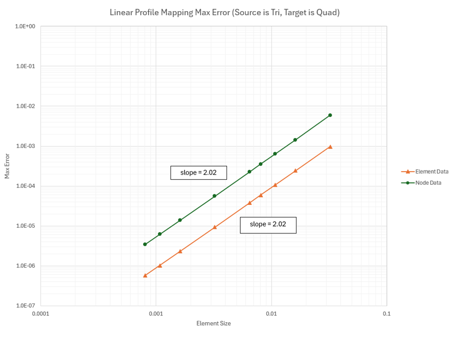
Figure 5: Mapping error plots
